Learning to Rank: The Hidden Layer Powering Modern RAG
In this article
- Why Ranking is Not Classification
- The Three Paradigms of LTR
- LambdaMART: The "Physics Trick"
- Implementation: LightGBM LambdaRank
- Measuring What Matters: Evaluation Metrics
- From DSSM to BERT: The Neural Revolution
- Cross-Encoders vs. Bi-Encoders
- Two-Stage Retrieval: The Production Standard
- Production Re-rankers: Your Options
- Fine-Tuning: Synthetic Data & Hard Negatives
- The LLM Revolution: RankGPT and RankRAG
- Framework Integration
- The Bigger Picture
Google, Netflix, ChatGPT with web search—what do they have in common? A ranking algorithm decides what you see first. It’s not about what exists; it’s about what surfaces. In the world of RAG (Retrieval-Augmented Generation), your pipeline is only as good as your ranker. Feed an LLM irrelevant context, and no amount of prompt engineering will save the output. The "R" in RAG is a ranking problem wearing a retrieval costume.

Why Ranking is Not Classification
Standard machine learning predicts a single value per instance (Spam/Not Spam). Ranking is different. Given a query and a set of documents, you must produce an optimal ordering where the most relevant items appear first. Absolute scores don't matter; relative ordering does.
Consider two models:
- Model A: Assigns 0.1 to a relevant document and 0.2 to an irrelevant one. (Wrong order, low score error).
- Model B: Assigns 0.7 to a relevant document and 0.5 to an irrelevant one. (Correct order, higher score error).
Model B wins. Users don't see scores; they see the list. This requires specialized loss functions that optimize for the quality of the ranked list itself.
The Three Paradigms of LTR
| Paradigm | Approach | Algorithms |
|---|---|---|
| Pointwise | Treats ranking as independent regression/classification per document. | Linear Regression, SVM. |
| Pairwise | Predicts which of two documents (A or B) should rank higher for a query. | RankNet, LambdaRank. |
| Listwise | Optimizes the entire ranked list directly (e.g., NDCG). | ListNet (Plackett-Luce), LambdaMART. |
LambdaMART: The "Physics Trick"
How do you optimize for a non-differentiable metric like NDCG? The breakthrough came with LambdaRank (2006) and LambdaMART (2010).
Instead of deriving gradients from a cost function (impossible for step functions), LambdaRank defines the gradients directly as the "forces" that push documents toward their correct positions.
The lambda gradient ($\lambda_{ij}$) for a document pair combines the pairwise gradient with the actual metric change: $$\lambda_{ij} = \sigma(s_j - s_i) \times |\Delta NDCG|$$
Where $|\Delta NDCG|$ is the improvement in the metric if documents $i$ and $j$ swapped positions. This bypasses non-differentiability by computing gradients after sorting.
Implementation: LightGBM LambdaRank
The group parameter is critical—it tells the ranker which documents belong to each query for list-aware optimization.
from lightgbm import LGBMRanker

# Initialize the ranker
ranker = LGBMRanker(
    objective="lambdarank",
    metric="ndcg"
)

# Fit the model
ranker.fit(
    X_train, y_train,
    group=query_doc_counts,  # [10, 15, 8] = 3 queries with 10, 15, 8 docs
    eval_set=[(X_val, y_val)],
    eval_group=[val_query_counts],
    eval_at=[5, 10]  # Optimize for NDCG@5 and NDCG@10
)
Measuring What Matters: Evaluation Metrics
1. NDCG (Normalized Discounted Cumulative Gain)
The gold standard. It handles graded relevance with logarithmic discounts for lower positions: $$DCG@k = \sum_{i=1}^{k} \frac{2^{rel_i} - 1}{\log_2(1+i)}$$
2. MRR (Mean Reciprocal Rank)
Answers: "On average, how far down is the first relevant result?" $$MRR = \frac{1}{|Q|} \sum_{i=1}^{|Q|} \frac{1}{rank_i}$$ If your RAG pipeline takes the top-1 result, MRR tells you how often that result is actually relevant.
3. MAP (Mean Average Precision)
Computes the area under the precision-recall curve for binary relevance.
From DSSM to BERT: The Neural Revolution
Before 2019, LTR relied on feature engineering (BM25, document length, PageRank).
- DSSM (2013): Pioneered neural ranking by mapping queries/docs into a shared semantic space. It learned "meaning" but often "forgot words" (product codes, technical terms).
- The BERT Jump (2019): Nogueira and Cho applied BERT to re-ranking, achieving a 27% relative MRR@10 improvement on MS MARCO—the largest single jump in history. The secret was Cross-Attention.
Cross-Encoders vs. Bi-Encoders
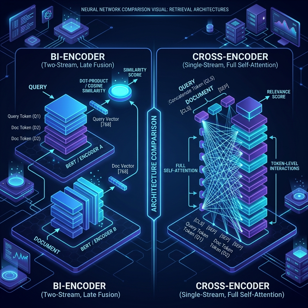
- Bi-Encoders: Separate encoders for query and doc. Scalable via ANN search (Vector DBs). Lower accuracy due to information loss in fixed-size vectors.
- Cross-Encoders: Query and doc are concatenated. Full cross-attention captures fine-grained interactions. Highly accurate but very slow (~5-20ms per doc).
Two-Stage Retrieval: The Production Standard
Modern RAG uses a two-stage approach:
- Stage 1: Fast Recall: Use Bi-Encoders or BM25 to retrieve the top 50-100 candidates from millions of chunks.
- Stage 2: Accurate Re-ranking: Apply a Cross-Encoder (like BGE or Cohere) to the top candidates to select the final 5-10 chunks.
Hybrid Retrieval (BM25 + Dense)
Combining keyword matching with semantic matching is non-negotiable. Use Reciprocal Rank Fusion (RRF) to merge results: $$score(d) = \sum \frac{1}{k + rank(d, retriever)}$$
Production Re-rankers: Your Options
1. Managed: Cohere Rerank 3.5
Handles 100+ languages, JSON, and tables.
import cohere
co = cohere.Client('api-key')
results = co.rerank(query="Node.js leaks", documents=chunks, model="rerank-v3.5", top_n=5)
2. Open-Source: BGE-M3 & Gemma
BGE (BAAI) offers state-of-the-art multilingual re-rankers like bge-reranker-v2-m3.
Fine-Tuning: Synthetic Data & Hard Negatives
Generic models often fail on domain-specific jargon.
- Synthetic Data: Use an LLM to generate plausible queries for your document chunks.
- Hard Negative Mining: The secret to precision. Random negatives are too easy. Hard negatives are documents that are "almost matches" but are technically irrelevant.
# Pseudo-code for hard negative mining
for query, positive_doc in training_data:
    candidates = retriever.search(query, top_k=20)
    hard_negatives = [doc for doc in candidates if doc != positive_doc and not is_relevant(query, doc)]
The LLM Revolution: RankGPT and RankRAG
- RankGPT: Demonstrates that GPT-4 can perform zero-shot ranking through instruction-based permutation.
- Distillation: Models like RankVicuna or RankZephyr distill GPT-4 intelligence into smaller, deployable 7B models.
- RankRAG (NeurIPS 2024): Instruction-tuning a single LLM for both ranking and generation. Unified models significantly outperform GPT-4 on knowledge-intensive tasks.
Framework Integration
LlamaIndex
from llama_index.core.postprocessor import SentenceTransformerRerank
reranker = SentenceTransformerRerank(model="BAAI/bge-reranker-v2-m3", top_n=5)
query_engine = index.as_query_engine(similarity_top_k=20, node_postprocessors=[reranker])
LangChain
from langchain.retrievers import ContextualCompressionRetriever
from langchain.retrievers.document_compressors import CrossEncoderReranker
compressor = CrossEncoderReranker(model=model, top_n=5)
compression_retriever = ContextualCompressionRetriever(base_compressor=compressor, base_retriever=vector_store.as_retriever(k=20))
The Bigger Picture
RAG systems are fundamentally ranking problems with generation attached. Mastering NDCG, lambda gradients, and cross-encoder tradeoffs is the only way to build AI applications that actually work at scale. Skip these, and you're building on sand.
Related Guides
Build a Local LLM Zero-Shot Classifier You Can Actually Deploy
Learn how to run zero-shot text classification on a local model with Ollama, enforce strict JSON outputs, and add confidence-aware routing for production triage.
The Complete Developer Guide to Running LLMs Locally: From Ollama to Production
Everything you need to run LLMs on your own hardware in 2026: VRAM sizing, model formats, an 8-tool comparison table, a full local RAG pipeline, and Docker production deployment with GPU passthrough and Nginx auth.
Event-Driven Architecture for Agentic AI: The Architect's Guide
A comprehensive architectural guide to designing resilient, real-time agentic AI systems using event-driven architecture — covering loose coupling, fault isolation, reference architecture, and governance patterns.